Finding Every Possible Pythagorean Triple

Pythagorean triples are sets of three integers which satisfy a very specific relationship—two of those integers form the base of a right triangle, with the third being the hypotenuse. There are many common ones, like $ (3, 4, 5) $, or $ (5, 12, 13) $, but as the numbers grow, finding these triples becomes a difficult task. Is it possible to procedurally generate these triples? To answer this question, we begin by examining what makes the relationship between integers in a Pythagorean triple unique.

Fermat’s Last Theorem #

In solving any type of mathematical problem, it’s often useful to connect it to more general problems, which can provide a bit of context to guide the solution process. The question of finding all possible Pythagorean triples is a good example of this. We are essentially asking to find $ A $, $ B $, and $ C $ such that:

$$ A^2 + B^2 = C^2 \space \textnormal{where} \space A, B, C \in \Z $$

As it happens, there are infinitely many $ A $, $ B $, and $ C $ such that this equation is true. Yet, perhaps a more subtle peculiarity is that the Pythagorean theorem is a very special case of a much larger problem, for which this property does not exist. If we consider the same problem in $ A $, $ B $, and $ C $ but simply change the exponent and ask for integer solutions:

$$ A^n + B^n = C^n \space \textnormal{where} \space A, B, C, n \in \Z \space \cap \space n > 2 $$

there are not infinite but zero non-trivial solutions, which is to say that there are zero solutions where all $ A, B, C \neq 0 $. This is Fermat’s Last Theorem, which states that the equation $ A^n + B^n = C^n $ has no solutions over the integers if $ n > 2 $. This simple statement is deceptively hard to prove; it took more than three centuries for a formal proof to be presented after Fermat’s initial proposition in 1637 AD.

While mathematically proving that this is true is quite hard, it’s relatively simple to see its implications when we study this problem from a visual perspective. To do that, we’ll need to plot this equation as some kind of curve on the Cartesian plane. While we could go ahead and plot this in three dimensions, we can make a clever substitution that will allow us to plot this curve in two dimensions. If we divide both sides by $ C^n $, we get:

$$ \left( \frac{A}{C} \right)^n + \left( \frac{B}{C} \right)^n = 1 $$

Now, we notice that both $ \frac{A}{C} $ and $ \frac{B}{C} $ are rational numbers, since both their numerators and denominators are integers. This means we can make the substitution:

$$ (x, y) = \left( \frac{A}{C}, \frac{B}{C} \right) $$

Now we are looking for solutions to the equation:

$$ x^n + y^n = 1 \space \textnormal{where} \space x, y \in \mathbb{Q} $$

For now, we’ll stick to the cases where $ n > 2 $. Graphing the equation for various values of $ n $ reveals two families of similar-looking curves: one where $ n $ is even and one where $ n $ is odd.

As we increase the value of $ n $, the curves resemble one of the two families of curves shown above, depending on whether $ n $ is even or odd. Larger values of $ n $ result in sharper corners and the graph taking a more box-like shape. Now, we turn back to the case where $ n = 2 $ and ask what makes this different from all the others:

$$ x^2 + y^2 = 1 $$

Well, as it turns out, the “Fermat curve” for $ n = 2 $ is not a Fermat curve at all but one of the most familiar geometric objects in all of mathematics: the unit circle. Combining this with our knowledge that there are infinitely many Pythagorean triples, we can deduce that there must be infinitely many points on the unit circle with $ x, y \in \mathbb{Q} $. We term such a point with rational coordinates a rational point on the unit circle.

Going in the other direction, given a rational point on the unit circle $ (x, y) $, we can rewrite $ x $ and $ y $ as fractions $ \frac{a}{b} $ and $ \frac{c}{d} $, respectively. We then have:

$$ \left( \frac{a}{b} \right)^2 + \left( \frac{c}{d} \right)^2 = 1 $$

Clearing denominators gives:

$$ (ad)^2 + (bc)^2 = (bd)^2 $$

This is a Pythagorean triple! We simply let:

$$ (A, B, C) = (ad, bc, bd) $$

Thus, there is a direct correspondence between rational points on the unit circle and Pythagorean triples. Finding one gives us the other. In other words, our question is no longer “find all Pythagorean triples” but instead “find all rational points on the unit circle.”

Rational Points on a Conic #

So far, we’ve reduced the problem of finding all possible Pythagorean triples to finding all rational points on the unit circle. If we find a rational point on the unit circle, then we know it corresponds to a unique Pythagorean triple. To be fair, this may not seem like much of a reduction: we’ve reduced a difficult problem to one that at first glance seems even harder: how do you find rational points on a curve? And, as if that wasn’t enough, how do you find every rational point? Just like the previous section, we’re going to generalize a bit in the hopes of relating this problem to others and in turn finding a pattern that will help reduce this problem to one that can be more easily solved.

Last section we ended by asking how to find every rational point on the unit circle. This chapter, we’re going to do a bit more; we ask: how do you find every rational point on a conic in its most general form? First, we have to be clear what we mean by a conic “in its most general form.” We typically think of conics as being the result of cross sections of a cone at different angles. From these cross sections, we get the four standard conics: circles, ellipses, parabolas, and hyperbolas. When we graph these figures in the Cartesian plane and account for rotation, they all have an equation of the form:

$$ A x^2 + B y^2 + C xy + D x + E y + F = 0 $$

for some coefficients $ A, B, C, D, E, F $ where $ AB \neq 0 $. In other words, conics are just algebraic curves (often called “algebraic varieties”) of degree $ 2 $. Here’s the graph of an arbitrary conic $ \mathcal{C} $: $ x^2 + y^2 + xy + x + y - 1 = 0 $:

For the purposes of our problem, we’ll assume that $ \mathcal{C} $ contains some rational point $ \mathcal{O} $ that we are aware of. In this case, $ \mathcal{O} $ is the point $(-1, 1) $. What we’re going to do is create a generating function for every other rational point on $ \mathcal{C} $ simply from knowing $ \mathcal{O} $.

One interesting observation that we can make is that if we know what one of the variables, say $ y $, is in terms of some linear function $ \ell $ of the other, we can substitute it into the equation of our conic to get a quadratic in just one variable. This roots of this resulting quadratic give us the intersections between the conic $ \mathcal{C} $ and the linear function $ \ell $. A nice property of quadratics is that the constant term $ c $ of a quadratic $ a x^2 + b x + c = 0 $ is always a constant multiple of the product of the two roots. This follows from the fact that, by the Fundamental Theorem of Algebra, any quadratic can be factored as:

$$ a x^2 + b x + c = a(x - r)(x - s) $$

for some roots $ r, s $. Multiplying out the factored form yields:

$$ a x^2 + b x + c = a x^2 - a(r + s) x + ars $$

Setting the constant terms equal to each other gives:

$$ c = ars $$

We’ll assume that both our conic and our linear expression of $ y $ in terms of $ x $ have solely rational coefficients so that this quadratic has rational coefficients as well. If we know one of the roots $ s $ is rational, then the other root $ r $ must also be rational as:

$$ r = \frac{c}{as} \space \textnormal{where} \space c, a, s \in \mathbb{Q} $$

To sum up our work so far as it is relevant to solving this problem, we know that if we can express $ y $ as a linear function of $ x $ with rational coefficients, then we can substitute $ y $ into the equation to get a quadratic in $ x $. And, if that quadratic happens to have one rational root $ x = s $, then its second root $ x = r $ must also be rational. Right now, this may seem a bit complicated and useless, but the first step should give us a hint as to what we need to do: write $ y $ as a linear function of $ x $.

A linear function has the form $ y = a x + b $, where we’ll assume $ a $ and $ b $ are rational coefficients so the resulting quadratic contains solely rational coefficients as well. We will refer to such a line as a “rational line” and any conic with rational coefficients as a “rational conic.” The key to our solution lies in choosing a line such that when this value of $ y $ is substituted into $ \mathcal{C} $, we get a quadratic in $ x $ with at least one rational root, thereby implying the existence of another rational root, giving us another point on the conic with a rational $ x $-coordinate.

As hinted at before, what we’re essentially doing when we substitute a linear equation $ \ell $ for $ y $ in $ \mathcal{C} $ is solving for the intersection between this line and the conic. In other words, the problem of finding a linear function such that its substitution into $ \mathcal{C} $ gives a quadratic in $ x $ with at least one rational root is equivalent to finding a line which intersects $ \mathcal{C} $ at some point with a rational $ x $-coordinate.

But we have a point just like that! Earlier, we defined $ \mathcal{O} $ as a rational point on $ \mathcal{C} $, meaning both its coordinates are rational. If we draw any line through $ \mathcal{O} $ that intersects $ \mathcal{C} $ at another point $ P $, we have a second root for $ x $ in the resulting quadratic. But since $ \mathcal{O} $ is a rational point, the quadratic already has one rational root, and therefore its second root must be rational as well, meaning the intersection $ P $ has a rational $ x $-coordinate. But, if our line is also rational, then we can find the corresponding $ y $-coordinate as $ a x + b $, meaning that a rational $ x $ implies a rational $ y $ for any point on the line. Therefore, our second intersection point has a rational $ x $-coordinate and a rational $ y $-coordinate, making it a rational point on $ \mathcal{C} $.

Here’s an example:

Drawing the rational line $ y = -2x - 1 $ through $ \mathcal{O} $ intersects the ellipse again, yielding a second rational point $ \left( \frac{1}{3}, -\frac{5}{3} \right) $. Graphically, it is easy to see that if we want to get all rational points on $ \mathcal{C} $, we need to draw every single rational line through $ \mathcal{O} $ so that we “sweep” through the entire plane. Mathematically speaking, we know that given two rational points, the line between them must have a rational slope, since their slope can be expressed as the quotient of their differences in $ x $ and $ y $, which are in turn rational. If we draw a line for every possible rational slope, we must inevitably find every rational point.

Our question now is simply how to parameterize the conic $ \mathcal{C} $ so that we account for all rational points and only the rational points. We call such a parametrization a “rational parametrization” of the conic $ \mathcal{C} $. Rational parametrizations parameterize a curve $ \mathcal{C} $ as a function of some rational variable $ t $ such that for every rational $ t $, a rational $ (x, y) $ coordinate pair is generated.

At this point, we could very well go ahead and parametrize $ \mathcal{C} $ in terms of the slope of our line, though a more geometrically pleasing way to think about this involves drawing a second rational line. Accounting for all slopes just means we need to pick a second point somewhere on the Cartesian plane that constantly moves so as to change the slope of our line continuously. We already know that the slope between two rational points is rational, so we just need to find a set of rational points on the plane that satisfy this condition of a continuously changing slope.

A rational line provides the perfect answer. By moving through every point on a rational line, we change the slope of the line intersecting the conic. That’s because two lines with distinct slopes intersect at one and only one point. In our example, one of the lines (the line from which we are choosing the set of points) never changes slope. Thus, in order for the intersection point to change, the line intersecting the conic must change slope. Traversing through all possible points on a rational line generates intersecting lines with all possible slopes (with one exception, as we’ll see later). A geometric diagram will make this intuitively clearer.

Our algorithm is as follows:

1. Pick a rational number $ t $ over which $ \mathcal{C} $ will be parameterized
2. Evaluate $ f(t) $ for some rational linear function $ f(x) = c x + d $ to yield some rational point $ Q $ on $ f $
3. Draw a line $ \ell $ through points $ \mathcal{O} $ and $ Q $, where $ \mathcal{O} $ is a rational point on $ \mathcal{C} $
4. Solve for the intersection $ \ell \cap \mathcal{C} $, which yields the desired corresponding rational point $ P $ on $ \mathcal{C} $

$ f(t) $ is plotted in green; $ t $ determines the point $ Q $ (in purple) on $ f $; the line connecting $ Q $ and $ \mathcal{O} $ is in blue and intersects the conic at point $ P $

In effect, we are “projecting” the conic $ \mathcal{C} $ onto $ f(t) $, which in turn forms a unique mapping between points on $ \mathcal{C} $ and points on $ f(t) $, which we exploit to rationally parametrize any conic. One final note that should be made before we move on to circles is that this method does not find every rational point; in particular, it misses exactly one point. This occurs at the point where the tangent line to the conic $ \mathcal{C} $ is exactly parallel to the line $ f(t) $ from which we are choosing $ Q $. This, in turn, means that the two lines never intersect and thus there is no point $ Q $ on $ f(t) $ that will correspond to this point on the conic. We introduce this more as a technicality than a severe issue as it presents no further problems later in our quest to find all Pythagorean triples. If you are curious as to whether it is possible to include this mysterious point in our parametrization, rest assured that it is indeed possible using the projective plane, where we say that this point corresponds to $ t = \infty $, though that is a subtlety that we will ignore.

The Weierstrass Substitution #

Hooray! 🎉 The hard work is (mostly) done. We needed to rationally parameterize the unit circle, yet instead we developed a rational parametrization for every conic. Now all we have to do is come up with an efficient way to apply what we’ve learned from the previous section to the unit circle.

To rationally parameterize a conic, we need two things: some rational point $ \mathcal{O} $ and some rational line to project the conic onto. In the case of the unit circle, we have four “obvious” rational points: $ (\pm 1, 0), (0, \pm 1) $. For reasons that will be made clear later, let’s choose the point $ (-1, 0) $ to be $ \mathcal{O} $. For our rational projection line, we have a myriad of options. However, though our previous example showed the rational line outside the conic, there is by no means any reason why our projection line cannot intersect the conic itself. Sometimes, the best options are the most obvious ones; in our case, those are the $ x $ and $ y $ axes themselves. We see immediately that the $ x $ axis does not work as no matter what point we choose, the line from $ (-1, 0) $ will have slope $ 0 $, and thus only intersect the circle at the point $ (1, 0) $. This leaves the $ y $ axis as the next easiest choice.

Moving to step two in our algorithm, we need to map some rational number $ t $ to a rational point along the $ y $ axis. We can easily do this by parameterizing the $ y $ axis as $ (0, t) $. This gives us our point $ Q $ for step three.

We now draw the line $ \ell $ through $ \mathcal{O} $ and $ Q $, which is given by the equation $ y = t(x + 1) $. The output of our algorithm, the intersection $ \ell \cap \mathcal{C} $, gives us the desired rational point $ P $. Substituting our definition of $ y $ from $ \ell $ into the definition of the unit circle yields:

$$ x^2 + t^2(x + 1)^2 = 1 $$

Rearranging gives:

$$ t^2(1 + x)^2 = 1 - x^2 $$ $$ t^2(1 + x)\cancel{(1 + x)} = \cancel{(1 + x)}(1 - x) $$ $$ t^2(1 + x) = 1 - x $$

At this point we can solve for $ x $ in terms of $ t $ to get:

$$ x = \frac{1 - t^2}{1 + t^2} $$

Substituting this into the definition of $ \ell $ yields a value for $ y $ as well:

$$ y = t \left( \frac{1 - t^2}{1 + t^2} + 1 \right) = t \left( \frac{2}{1 + t^2} \right) = \frac{2t}{1 + t^2} $$

Combining these two equalities yields the rational parametrization of the unit circle:

$$ (x, y) = \left( \frac{1 - t^2}{1 + t^2}, \frac{2t}{1 + t^2} \right) $$

We see immediately that for any $ t \in \mathbb{Q} $, we must get a corresponding rational point on the unit circle, as generating this point consists only of multiplication, division, addition, and subtraction, which, when applied to rational numbers, always yield a rational number as an output. Note that this is not the case if we use the familiar parametric equation of a circle $ (\cos \theta, \sin \theta) $; even if we have $ \theta \in \mathbb{Q} $, we cannot guarantee that the output of either $ \cos \theta $ or $ \sin \theta $ will yield a rational output (try expressing the point $ (\cos 1, \sin 1) $ in terms of rational coordinates).

While our result is obviously important algebraically, it can also be quite powerful to look at it from a geometric perspective.

Points on the unit circle are projected onto the $ y $ axis, with points in the first and fourth quadrants being mapped to points inside the unit circle (where $ -1 \leq t \leq 1 $) and points in the second and third quadrants being mapped to points outside the unit circle (where $ |t| > 1 $).

What we’re going to do now is not directly related to our problem of finding all possible Pythagorean triples, so feel free to skip over to the next section. However, the process which we’re about to explore is so important that it is in many ways impossible to skip now that we’ve covered the rational parametrization of the unit circle.

Earlier it was hinted at that of the four rational points that we could have chosen as $ \mathcal{O} $, there was a reason why $ (-1, 0) $ was chosen in particular. That reason, as we can see now, is that $ t $ becomes the slope of the line $ \ell $, which makes the math we’re about to do much simpler. We’re going to explore the answer to a very obvious next question which is: how do we relate the rational parametrization of the circle to its traditional parametrization as $ (\cos \theta, \sin \theta) $? More specifically, we’re going to ask the question:

Given a point in the form $ (\cos \theta, \sin \theta) $ for some angle $ \theta $, what is the corresponding value of $ t $ that will generate that point in our rational parametrization?

In fact, we’re going to forget about the condition $ t \in \mathbb{Q} $ that we imposed to ensure our parametrization produced only rational points and instead extend the domain of $ t $ to $ t \in \R $. To take a more geometric perspective, we are trying to find the value $ t $ shown in the diagram below:

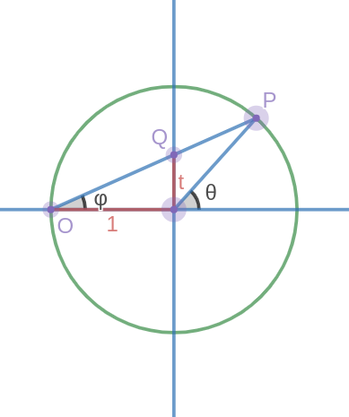
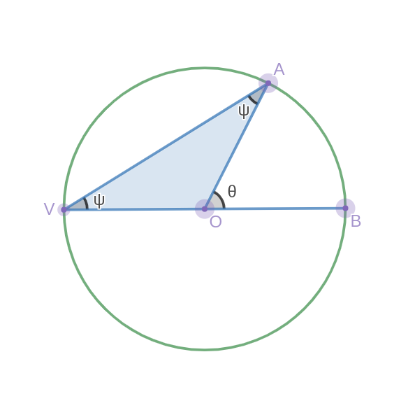
As the distance from our rational point $ (-1, 0) $ to the origin is just 1, we can use the tangent of $ \varphi $ to find $ t $. Now all we have to do is express $ \varphi $ in terms of $ \theta $. If you’re familiar with geometry, you’ll notice that $ \varphi $ is simply an inscribed angle and is therefore half the angle $ \theta $. A quick proof of this theorem is shown below (for the case where one chord is the diameter, as it is in our diagram):

Therefore:

$$ t = \tan \varphi = \tan \frac{\theta}{2} $$

Now we can equate our two parametrizations:

$$ (\cos \theta, \sin \theta) = \left( \frac{1 - t^2}{1 + t^2}, \frac{2t}{1 + t^2} \right) \space \textnormal{where} \space t = \tan \frac{\theta}{2} $$

Okay, so what? We already knew that both parametrizations described the same object, so what’s the point in equating them? For that matter, why didn’t we go the other way around and ask to express our parametrization in terms of the common $ (\cos \theta, \sin \theta) $ by finding a value for $ \theta $ in terms of $ t $? As a matter of fact, that’s what we’ll do quite shortly, though in a slightly different way. However, the key reason that this equation is so important is because it gives us an alternate way to express the trigonometric functions $ \cos x $ and $ \sin x $:

$$ \textnormal{Let: } t = \tan x/2 $$ $$ \sin x = \frac{2t}{1 + t^2} $$ $$ \cos x = \frac{1 - t^2}{1 + t^2} $$

In other words, not only have we characterized the unit circle in terms of $ t $ but also the trigonometric functions of $ \sin $ and $ \cos $. We can now express the two most elementary trigonometric functions in terms of a single parameter $ t $, which in turn allows us to express any of the six fundamental trig functions in terms of $ t $ as well. This substitution is known as the “Weierstrass substitution,” hence the name of this section.

To understand what this means and why it’s so important, take the fairly complex trig identity:

$$ \frac{\cos^{4} x -\sin^{4} x}{\cos^{2}x} = 1-\tan^{2}x $$

Your first instinct is probably to try and factor to get rid of the annoying $ \sin x $ term and then hope everything simplifies to yield a $ \tan^{2}x $ term somehow. But what if all three trigonometric functions could be expressed in terms of a single variable $ t $? Then the problem simply becomes algebra: simplify the rational functions of $ t $ on both sides and show they’re equivalent. Here’s what it would look like if we expressed everything in terms of $ t $ using the Weierstrass substitution and then wrote the left and right sides as rational functions:

$$ \frac{\left(1-t^{2}\right)^{4}-\left(2t\right)^{4}}{\left(1-t^{2}\right)^{2}\left(1+t^{2}\right)^{2}} = 1-\frac{\left(2t\right)^{2}}{\left(1-t^{2}\right)^{2}} $$

Combining the right side into one fraction yields:

$$ \frac{\left(1-t^{2}\right)^{2}-\left(2t\right)^{2}}{\left(1-t^{2}\right)^{2}} $$

Clearing the denominator on the right side gives:

$$ \frac{\left(1-t^{2}\right)^{4}-\left(2t\right)^{4}}{\left(1+t^{2}\right)^{2}} = \left(1-t^{2}\right)^{2}-\left(2t\right)^{2} $$

Clearing denominators yet again, this time on the left side, yields:

$$ \left(1-t^{2}\right)^{4}-\left(2t\right)^{4} = \left(1+t^{2}\right)^{2}\left(\left(1-t^{2}\right)^{2}-\left(2t\right)^{2}\ \right) $$

At this point, we can simply expand all the binomials to get:

$$ 1-4t^{2}-10t^{4}-4t^{6}+t^{8} = \left(1+2t^{2}+t^{4}\right)\left(1-6t^{2}+t^{4}\right) $$

Performing long division proves that this is indeed the correct factorization of the polynomial on the left, and therefore the identity must be true. While this process does of course involve significantly more algebra than the traditional approach to proving trig identities, it is an immensely powerful tool in solving them because it provides a way to turn problems in trigonometry into problems of algebra, thereby allowing for a systematic approach to proving that a given identity is either true or false.

As a matter of fact, these identities are extremely powerful tools in calculus as well. Say we wanted to evaluate the indefinite integral:

$$ \int \csc x \space dx $$

We could very well express this in terms of $ \sin x $ to get:

$$ \int \frac{dx}{\sin x} $$

but this gets us nowhere—that is until we use the Weierstrass substitution. To do that, however, we’ll need to express $ x $ in terms of $ t $ to replace the $ dx $ term and integrate over $ t $. Recall from our definition of $ t $ that we have:

$$ t = \tan x/2 \Rightarrow x = 2 \arctan t $$

This is essentially the Weierstrass substitution in reverse: it gives us a way to write the rational parametrization in terms of the traditional $ (\cos \theta, \sin \theta) $ parametrization of the unit circle. Using this to rewrite our integral gives:

$$ \int \frac{1 + t^2}{2t} \space d(2 \arctan t) = \int \frac{1 + t^2}{2t} \space \frac{d}{dt}(2 \arctan t) \space dt $$

Multiplying by the derivative of $ 2 \arctan t $ yields a rational expression in terms of $ t $ that we can integrate:

$$ \int \frac{\cancel{1 + t^2}}{2t} \cdot \frac{2}{\cancel{1+t^{2}}} \space dt = $$ $$ \int \frac{\cancel{2}}{\cancel{2}t} \space dt = \int \frac{dt}{t} $$

Aha! We’ve reduced the problem to a common integral. We can now integrate and substitute $ t = \tan x/2 $ to get:

$$ \int \frac{dt}{t} = \ln |t| = \ln |\tan x/2| $$

Viola! The Weierstrass substitution transformed the integral into a common form over which we could integrate and then substitute $ t = \tan x/2 $ to get a solution.

The Primitives #

At long last, we return again to the question of finding all possible Pythagorean triples. We’ve discussed Fermat curves and the peculiarity of the Pythagorean theorem, the rational parametrization of conics, and most recently the Weierstrass substitution, and we’re finally able to solve the problem of finding all Pythagorean triples.

We start by noting the most obvious way to generate a new Pythagorean triple: if we have some triple $ (A, B, C) $, then we can simply generate a new triple $ (tA, tB, tC) $ for some integer $ t $. However, these triples aren’t all that useful and are ultimately the result of the “base” triple $ (A, B, C) $. In other words, if we can find all of the triples $ (A, B, C) $ where $ A, B, C $ have no common factor (that is to say $ \gcd(A, B, C) = 1 $), then we can find all the other triples simply by multiplying by an integer $ t $. For now we’ll focus our attention on the “base” triples, which we’ll term “primitive” Pythagorean triples.

As a final restriction, we’ll note an interesting property that all primitive Pythagorean triples share: they always contain one even and one odd $ A $ or $ B $ term. To prove this, we’re going to have to leverage a bit of elementary number theory. The first case is that both $ A $ and $ B $ are even. We seek to force a contradiction that would require $ A $, $ B $, and $ C $ to have a common factor. If we consider this scenario under modulo $ 2 $, we get:

$$ A^2 + B^2 \equiv 0^2 + 0^2 = 0 \equiv C^2 \mod 2 $$ $$ A \equiv B \equiv C \equiv 0 \mod 2 $$

That last part follows from the fact that if $ 2 \mid C^2 $, since $ 2 $ is prime, we must also have $ 2 \mid C $. Thus, we’ve proven that $ A $, $ B $, and $ C $ must all be even, therefore meaning that the triple is not primitive (all are divisible by $ 2 $), and thus ruling out that possibility. The next case requires proving that it is impossible for both $ A $ and $ B $ to be odd. We consider the situation under modulo $ 4 $:

$$ A^2 + B^2 \equiv \set{ 1, 3 }^2 + \set{ 1, 3 }^2 \equiv 1 + 1 = 2 \equiv C^2 \mod 4 $$

* The set notation $ \set{} $ is used here to indicate all possibilities of congruence

What the above equation tells us is that $ C^2 $ must be divisible by 2, but not by 4. Yet if $ C^2 $ is divisible by 2, since 2 is prime it must also divide $ C $ itself. But if 2 divides $ C $, then $ 2 \times 2 $ divides $ C^2 $ which thereby implies that $ 4 $ divides $ C^2 $, the contradiction we were looking for. Thus, every primitive Pythagorean triple must have one even and one odd $ A $ or $ B $. For the rest of this section we will assume $ A $ to be odd and $ B $ to be even.

As pointed out in the first section, any Pythagorean triple $ (A, B, C) $ can be transformed onto the unit circle as the point $ (x, y) = (A/C, B/C) $ (primitive triples and their multiples are represented as the same point). What this means is that every possible primitive Pythagorean triple corresponds to a unique rational point on the unit circle; if we find all the rational points on the unit circle, we’ve found all the Pythagorean triples. But we know how to do that!

At this point, we could certainly use the rational parametrization of the unit circle we derived earlier to find all the Pythagorean triples. However, we’re going to restrict ourselves to generating only the primitive Pythagorean triples. Notice also that if we were to simply use the rational parametrization as is, we would end up with a lot of non-primitive triples for $ |t| > 1 $ and a lot of fractional ones for $ |t| < 1 $ (which aren’t really triples at all since $ A, B, C \notin \Z $).

The key insight is to let $ t = p/q $ for some integers $ p $ and $ q $. Expressing $ t $ in “rational” form allows us to express the result in a similar rational form, from which we can generate a non-fractional Pythagorean triple. Substituting $ t = p/q $ into the rational parametrization of the unit circle gives:

$$ \left(\frac{q^{2}-p^{2}}{q^{2}+p^{2}},\frac{2pq}{q^{2}+p^{2}}\right) $$

We quickly see that for all $ p < q $, we get a series of three integers which is a Pythagorean triple: $ (q^2-p^2, 2pq, q^2+p^2) $. Note that $ p < q $ is not really a limitation as it only serves to ensure that all the triples we generate have positive values for $ A, B, C $.

Now all that’s left is to rigorously prove that the above Pythagorean triple is always primitive no matter the choice of $ p $ and $ q $. However, since we’re expressing $ t $ in simplest form so as to avoid duplicates, $ p $ and $ q $ must be relatively prime, which is the first restriction we will impose before we carry out the proof. The last restriction is that, in order for $ A $ to be odd like we assumed, we must have $ 2 \nmid (q^2 - p^2) $, which forces one of $ p $ and $ q $ to be even and the other to be odd. Summing up all our restrictions, we have:

1. Domain: $ p, q \in \mathbb{Z}^{+} $
2. Positivity: $ p < q $
3. Relative Primality: $ \gcd(p, q) = 1 $
4. Even/Odd Split: $ (2 \mid p \cap 2 \nmid q) \cup (2 \nmid p \cap 2 \mid q) $

Now we proceed to prove that the triple $ (q^2-p^2, 2pq, q^2+p^2) $ is indeed primitive. We begin without assuming that this generated triple is primitive. Instead, let it be a constant multiple $ \lambda $ of some primitive triple $ (A, B, C) $ such that:

$$ \lambda A = q^2 - p^2 $$ $$ \lambda B = 2pq $$ $$ \lambda C = q^2 + p^2 $$

If we can show that $ \lambda = 1 $, then we’ve successfully proven that the triple is primitive, since that would mean our primitive triple $ (A, B, C) $ exactly equals the desired values. Since $ A, B, C \in \mathbb{Z} $, $ \lambda $ must divide the terms on the right hand side of these expressions. Thus, we have:

$$ \lambda \mid q^2 - p^2 $$ $$ \lambda \mid 2pq $$ $$ \lambda \mid q^2 + p^2 $$

The first and third expressions are particularly interesting; since $ \lambda $ divides them both, it must also divide their sum and difference. This gives us:

$$ \lambda \mid 2q^2 $$ $$ \lambda \mid 2p^2 $$

If $ \lambda $ were to divide both $ p^2 $ and $ q^2 $, then at least one of its prime factors would have to be shared across $ p $ and $ q $; but this contradicts our third assumption that $ p $ and $ q $ must be relatively prime. Thus $ \lambda $ must divide $ 2 $. This in turn leaves us with only two options for $ \lambda $, which greatly narrows down the space of possible values to just the factors of two: $ 1, 2 $.

We now assume that $ \lambda = 2 $ and search for a contradiction. We know that $ A $ is odd, so we must have $ A \equiv 1 \space \mathrm{mod}\ 2 $. This gives:

$$ \lambda A = 2A \equiv 2 \mod 4 $$

Aha! We’ve seen this before! In our proof that both $ A $ and $ B $ could not be odd, we showed that it is impossible for the square of an integer to be congruent to $ 2 \space \mathrm{mod}\ 4 $. We have a similar definition for $ \lambda A $ that we can exploit:

$$ \lambda A = q^2 - p^2 \equiv 2 \mod 4 $$

Instead of proving that the square of an integer cannot be congruent to $ 2 \space \mathrm{mod}\ 4 $, we need to prove that the difference of the squares of two integers cannot be congruent to $ 2 \space \mathrm{mod}\ 4 $. The process is nearly identical; we have*:

$$ q^2 - p^2 \equiv \set{0,…,3}^2 - \set{0,…,3}^2 \equiv \set{0,1} - \set{0,1} = \set{0,-1,1} \mod 4 $$

*We could have also applied the restriction that only one of $ p $ and $ q $ is even, but this is not necessary to complete the proof

When we simplify the set so as to contain only positive integers the contradiction is immediately apparent:

$$ 2 \notin \set{0,1,3} $$

Thus, the difference of the squares of two integers cannot be congruent to $ 2 \space \mathrm{mod}\ 4 $, and in turn $ \lambda $ cannot equal $ 2 $, which means $ \lambda = 1 $, as desired.

✨ We’ve proven that the triple $ (q^2-p^2, 2pq, q^2+p^2) $ is primitive!

On the Cartesian Plane #

At long last, we finally have a generative algorithm for finding every possible primitive Pythagorean triple, which in turn gives us every Pythagorean triple by multiplying the entire triple by an integer constant. Our algorithm essentially does the following:

1. Pick some integer $ q \in \mathbb{Z}^{+} $
2. Pick some positive integer $ p $ of opposite parity to $ q $ where $ p < q \space \cap \space \gcd(p, q) = 1 $
3. Generate the primitive triple $ (A, B, C) = (q^2 - p^2, 2pq, q^2 + p^2) $
4. Multiply by a constant $ k \in \mathbb{Z}^{+} $ to generate all derived triples $ (kA, kB, kC) $

To implement this in Python code, we’re going to stick to generating only the primitive triples (steps 1-3) over a given range for $ p $ and $ q $. First, we code the generator:

def generate(p, q):
    A = q ** 2 - p ** 2
    B = 2 * p * q
    C = q ** 2 + p ** 2
    return A, B, C

Now, we run two loops: one where we test for all primitive triples with p even and q odd and the other where the reverse is true. We’ll need the math library to check for the greatest common divisor and then write two nested for loops which traverse a range from 1 to some upper bound limit:

for q in range(1, limit, 2):  # skips all even integers (q is odd)
    for p in range(2, q, 2):  # skips all odd integers (p is even)
        if math.gcd(p, q) == 1:
            A, B, C = generate(p, q)
            print(A, B, C)

for q in range(2, limit, 2):  # skips all odd integers (q is even)
    for p in range(1, q, 2):  # skips all even integers (p is odd)
        if math.gcd(p, q) == 1:
            A, B, C = generate(p, q)
            print(A, B, C)

Putting this all together, we have:

import math

# Write limit here!
limit = ...

def generate(p, q):
    A = q ** 2 - p ** 2
    B = 2 * p * q
    C = q ** 2 + p ** 2
    return A, B, C

for q in range(1, limit, 2):
    for p in range(2, q, 2):
        if math.gcd(p, q) == 1:
            A, B, C = generate(p, q)
            print(A, B, C)

for q in range(2, limit, 2):
    for p in range(1, q, 2):
        if math.gcd(p, q) == 1:
            A, B, C = generate(p, q)
            print(A, B, C)

Running this with limit = 100 gives triples as obscure as $ (5811, 10340, 11861) $ and some with a difference of just $ 1 $ between two of the numbers, like $ (195, 19012, 19013) $. As a final step, we’re going to plot a finite number of these triples on the Cartesian plane with coordinates $ (A, B) $ and distance $ C $ from the origin, which will be shown with a line from the origin to each point. We’ll use limit=20, which gives us $ 78 $ distinct triples. At this point, we turn to matplotlib to handle the plotting aspect of our algorithm. We then modify our original code to store all the triples to a list instead of immediately printing them:

import matplotlib.pyplot as plt
from matplotlib import collections as mc

limit = 20
triples = []

def generate(p, q):
    A = q ** 2 - p ** 2
    B = 2 * p * q
    C = q ** 2 + p ** 2
    return A, B, C

for q in range(1, limit, 2):
    for p in range(2, q, 2):
        if math.gcd(p, q) == 1:
            A, B, C = generate(p, q)
            triples.append((A, B, C))

for q in range(2, limit, 2):
    for p in range(1, q, 2):
        if math.gcd(p, q) == 1:
            A, B, C = generate(p, q)
            triples.append((A, B, C))

We then create a matplotlib figure that we can add to. We will define two lists to store the coordinates of each triple and then a third list to store a collection of line segments that we turn into a matplotlib.collections.LineCollection object:

fig = plt.figure(figsize=(10, 10), dpi=200)
x = [triple[0] for triple in triples]
y = [triple[1] for triple in triples]
lines = [[(0, 0), (x[i], y[i])] for i in range(len(x))]
figLines = mc.LineCollection(lines, colors=(0.25, 0.33, 0.67, 0.25), linewidths=1)

We now add our line collection to a subplot and create a scatter plot which holds our points. After some formatting to position the axes, the final part of our code looks like:

ax = fig.add_subplot(1, 1, 1)
ax.set_title('All primitive Pythagorean triples')
ax.add_collection(figLines)
ax.scatter(x, y, s=5, color=(0.25, 0.33, 0.67, 1))

ax.spines.left.set_position('zero')
ax.spines.right.set_color('none')
ax.spines.bottom.set_position('zero')
ax.spines.top.set_color('none')
ax.xaxis.set_ticks_position('bottom')
ax.yaxis.set_ticks_position('left')
ax.autoscale()

plt.show()

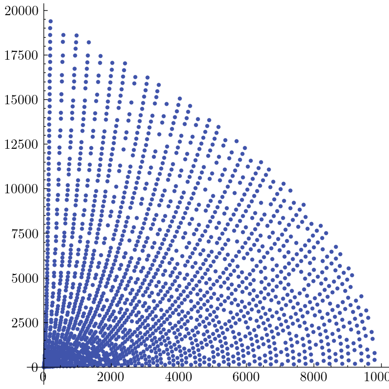
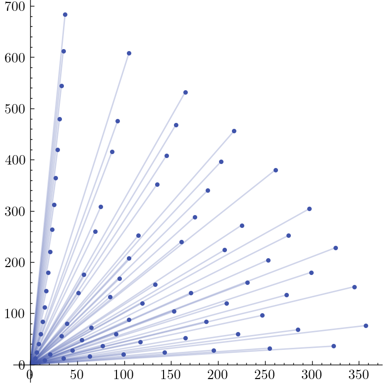
🎊 Finally, we can see the results of our algorithm! Running the full program and capturing the result produces a truly outstanding final plot, revealing an interesting structure to the Pythagorean triples:

Plotted with style SciencePlots

Here’s an interactive demo where you can set different limit values and see the results change:

For the grand finale, here’s what plotting the first $ 2000 $ primitive Pythagorean triples looks like (with limit=100 and no lines to reduce clutter):